Sagitta
Scott Prahl
Jan 2023
[1]:
%config InlineBackend.figure_format = 'retina'

import sys
import numpy as np

if sys.platform == "emscripten":
    import piplite

    await piplite.install("lenstest")

from lenstest.lenstest import sagitta
Conic Sections
Optical surfaces are typically spherical, however a number of other shapes occur. For telescope mirrors, a parabolic shape is preferred. In general, these shapes are commonly described by conic sections. The conic curves can be described by a conic constant K

where the numbers in the plot indicate the values of the conic constant for different curves.
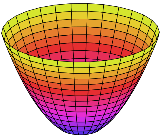
The mirror surfaces are formed by rotating about and optical axis oriented perpendicular to the vertex. So a paraboloid mirror might look like
Sagitta
The height (or depth) of a convex or concave lens surface is referred to as the sagitta, or simply sag, of that surface.
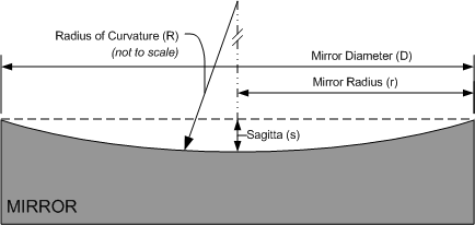
The sagitta for a conic section is given by the radius \(r\) of the chord distance \(2r\), the radius of curvature of the section \(R\), and the conic constant K:
Testing Sagitta Calculations
To check the calculations of sagitta for different conic sections, this paper about contact lens calculations was handy. This paper by Benjamin & Rosenblum was useful: “Radii of Curvature and Sagittal Depths of Conic Sections”, International Contact Lens Clinic, Vol. 19, pp. 76-83, March/April 1992. Specifically, the data from table 1 allows direct comparison with the understanding that the conic constant \(K\) is related to the eccentricity \(\varepsilon\) by
To get a positive conic constant, the eccentricity must be imaginary. Moreover, to the positive conic constant results to match, I modified the eccentricity from -0.45j to -0.504j
[2]:
RoC = 7.8  # mm
eccentricity = np.array([0.504j, 0, 0.45, 1, 2])
conic_constant = (-(eccentricity**2)).real

# table from the magazine
table_1 = np.array(
    [
        [1.0, 0.016, 0.016, 0.016, 0.016, 0.016],
        [2.0, 0.064, 0.064, 0.064, 0.064, 0.063],
        [3.0, 0.146, 0.146, 0.145, 0.144, 0.140],
        [4.0, 0.262, 0.261, 0.260, 0.256, 0.245],
        [5.0, 0.414, 0.412, 0.409, 0.401, 0.374],
        [6.0, 0.606, 0.600, 0.595, 0.577, 0.524],
        [7.0, 0.842, 0.829, 0.820, 0.785, 0.693],
        [8.0, 1.128, 1.104, 1.086, 1.026, 0.878],
        [9.0, 1.472, 1.429, 1.340, 1.298, 1.076],
        [10.0, 1.890, 1.813, 1.761, 1.603, 1.285],
        [11.0, 2.403, 2.269, 2.183, 1.939, 1.504],
        [12.0, 3.061, 2.816, 2.673, 2.308, 1.731],
    ]
)

y = (table_1[:, 0] / 2).flatten()  # heights
x = np.zeros_like(y)  # optical axis crosses conic at (0,0)RoC = 7.8

print('Benjamin & Rosenblum, "Radii of Curvature and Sagittal Depths of Conic Sections,')
print("ICLC, Vol. 19, pp. 76-83, March/April 1992")
print()
print("Radius of curvature is %4.1f mm" % RoC)
print("Nominal diameter of contact lens is %4.1f mm" % 12)
print()
print("Sagittal depths for conoid surfaces with fixed apical radius of curvature,")
print("for with different eccentricities. 2h is the chord length across")
print("the curved surface.")
print()
print(" 2h    e=-0.45   0.0   0.45    1.0     2.0")
for i in range(len(x)):
    print(
        "%6.3f %6.3f %6.3f %6.3f %6.3f  %6.3f"
        % (2 * y[i], table_1[i, 1], table_1[i, 2], table_1[i, 3], table_1[i, 4], table_1[i, 5])
    )
Benjamin & Rosenblum, "Radii of Curvature and Sagittal Depths of Conic Sections,
ICLC, Vol. 19, pp. 76-83, March/April 1992

Radius of curvature is  7.8 mm
Nominal diameter of contact lens is 12.0 mm

Sagittal depths for conoid surfaces with fixed apical radius of curvature,
for with different eccentricities. 2h is the chord length across
the curved surface.

 2h    e=-0.45   0.0   0.45    1.0     2.0
 1.000  0.016  0.016  0.016  0.016   0.016
 2.000  0.064  0.064  0.064  0.064   0.063
 3.000  0.146  0.146  0.145  0.144   0.140
 4.000  0.262  0.261  0.260  0.256   0.245
 5.000  0.414  0.412  0.409  0.401   0.374
 6.000  0.606  0.600  0.595  0.577   0.524
 7.000  0.842  0.829  0.820  0.785   0.693
 8.000  1.128  1.104  1.086  1.026   0.878
 9.000  1.472  1.429  1.340  1.298   1.076
10.000  1.890  1.813  1.761  1.603   1.285
11.000  2.403  2.269  2.183  1.939   1.504
12.000  3.061  2.816  2.673  2.308   1.731
Here we verify that all these values can be calculated correctly.
[4]:
# now calculate and print these values

K = (-(eccentricity**2)).real
sag = np.zeros((12, 6))
sag[:, 0] = table_1[:, 0]

for i in range(len(K)):
    sag[:, i + 1] = sagitta(RoC, K[i], x, y)

print()
print("Sagitta calculated using sagitta()")
print()
print(" 2h    e=-0.45   0.0   0.45    1.0     2.0")
for i in range(len(x)):
    print(
        "%6.3f %6.3f %6.3f %6.3f %6.3f  %6.3f"
        % (sag[i, 0], sag[i, 1], sag[i, 2], sag[i, 3], sag[i, 4], sag[i, 5])
    )
Sagitta calculated using sagitta()

 2h    e=-0.45   0.0   0.45    1.0     2.0
 1.000  0.016  0.016  0.016  0.016   0.016
 2.000  0.064  0.064  0.064  0.064   0.063
 3.000  0.146  0.146  0.145  0.144   0.140
 4.000  0.262  0.261  0.260  0.256   0.245
 5.000  0.414  0.411  0.409  0.401   0.374
 6.000  0.606  0.600  0.595  0.577   0.524
 7.000  0.842  0.829  0.820  0.785   0.693
 8.000  1.128  1.104  1.086  1.026   0.878
 9.000  1.472  1.429  1.398  1.298   1.076
10.000  1.890  1.813  1.761  1.603   1.285
11.000  2.403  2.269  2.183  1.939   1.504
12.000  3.061  2.816  2.673  2.308   1.731
[ ]: